Julieta's GIS Blog

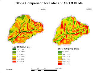
This was the first week addressing the topic of scale. The lab objective was to observe the effects of scale and resolution in spatial data properties for vector and raster data. First part of the lab required me to analyze differences in scale for hydrology features. Second, I had to compare two digital elevation models (DEMs), Lidar and SRTM, and figure out a method for comparing elevation data. I performed Slope, Aspect and Curvature analysis on the Lidar DEM at a resolution of 90m. Then performed Slope, Aspect, and Curvature analysis on the reprojected SRTM DEM also at 90m. This data allowed me to produce a chart listing averages for both DEMs in order to observe any trends. Notable inconsistencies were found in Average Slope degrees and Max elevation between the two DEMs. SRTM DEM had a lower measure at 29.4 average slope degrees, while the Lidar DEM was 31.3. Maximum elevation was higher for the Lidar DEM at 1063.05 than the SRTM DEM at 1053. DEM DEM resolution (mete

This week we were introduced to Geographically Weighted Regression (GWR). The main differences between a GWR and an Ordinary Least Squares (OLS) regression are: Where OLS is a global model, GWR is local Distances are NOT considered in OLS, whereas distances define the data fitting GWR Coefficients are constant in OLS, while in GWR they vary by location I was a lot more comfortable making these regressions and comparing for best fit variable models this time around. The lab consisted first of an example in comparing an OLS and GWR analysis and learning about the significance of differences in their prediction values. The second part another OLS and GWR analysis, this time I worked somewhat 'off-rails'. The exercise started by selecting a crime type, I chose 'Residential burglary', then making it a feature class in order to continue an analysis to find out what types of variables had the strongest correlation to high 'Residential burglary' rates in

The goal of this week's lab is to perform a series of multivariate regression analysis, examine and work with sophisticated diagnostics, and perform a regression analysis in ArcGIS. Last week's lab exercises served as a great refresher in basic statistics and introduction to simple regression analysis, which came in extremely useful in working through this lab. It involved a higher level of statistics comprehension. I started by carrying out a multivariate regression in Excel. Then compared multivariate models created in Excel. The last part of this lab required to use ArcGIS to perform an Ordinary Least Squares (OLS) analysis and regression diagnostics. I ran the OLS and Spatial Autocorrelation (Global Moran's I) tools three times to arrive at my final results for the best fit model. According to value result guidelines, I need to use the best fit model which consist of the highest Adjusted R-square and lowest AICc values. The first model that passed in Summary 4/8 con

This week we had to produce a classified image from satellite data using the supervised image classification method. To do this, first, I identified fourteen land cover types based on an original satellite image for Germantown, Maryland using the Inquire Cursor and Signature Editor in ERDAS Imagine. Then modified the band colors to better suit the features being represented. From there, I re-coded each class down to have eight as there were a few land cover types that repeated. This process required to create two additional images that incorporated these classes: a supervised image, and a distance image. I did another color pass in the new supervised since it is easier to have unique colors for eight classes. The final part of this map was completed in ArcMap, both of my own new images are represented here. While the supervised image displays the required eight land cover types, the distance image serves to show feature variances in color. The features with the brightest pixels he

This lab served as a great review of basic Statistics methods, then focusing on interpreting Regressions and Correlations. We started by reviewing basic Statistical functions in Excel, such as how to calculate Average, Median, Standard Deviation, etc. Then were introduced to the Data Analysis tool in Excel, which is super helpful in performing Descriptive Statistics, Correlations, and Regressions on different data sets from the lab. I’ve only ever taken an Introduction to Statistics course in College, so much of what we covered I recall having to do by hand on graph paper and calculator, fun times!... I see now that we will likely be performing some estimates in the case of missing data points. So I’m glad we got to cover this scenario in the last exercise in which we had to fill in estimated data using the Slope formula covered in lecture. I used the Slope formula Y = b*x + a in which b is the is the Slope .84, and a is the intercept coefficient 161.83, and x was my B column val

This lab wraps up our modules to do with Surface analyses. Our first objective was to calculate and interpret the vertical accuracy of a DEM using NDEP accuracy guidelines. The second objective was to observe the effects of interpolation methods on a DEM's accuracy. In the first accuracy analysis sample points appeared to be laid out in clusters instead of a natural distribution in which certain Land Cover types exhibit common areas. I’m leaning towards estimated interpolation causing this type of distribution because there is a notable gap of data points in higher elevation areas. I was able to plot a total of 2387 points from a provided table using the Make XY Event Layer tool. Then clipped the data points to the DEM extent. In order to be able to perform an analyses of the DEM and the reference point dataset, I extracted elevation values from the DEM and created a new set of points using the Extract values to Points tool. Then used the Extract Multi Values to Points tool