Julieta's GIS Blog

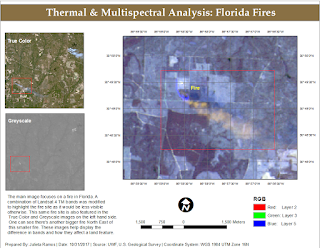
In our lab this week we delved more into Multispectral Analysis involving Thermal Imagery in order to learn how to interpret radiant energy. Using both ArcMap and ERDAS Imagine, I was able to create two different composite multispectral satellite images from TIFF files. For the final map assignment, I used the composite image created in Exercise 2 of this lab which I compiled in ERDAS Imagine. I had already identified a big fire site and then happened to find another one further down the image. As means to highlight the fire I modified the RGB bands to R-2, G-3, B-5 in the Landsat 4 TM satellite image. This made surrounding vegetation a dull blue while making the fire and its smoke orange.

Interpolation is utilized in order to give a raster cell a predicted number value. We use interpolation methods to create a value for unknown values basically. This is necessary for a number of different data gathering issues such as difficult environments or complex point data that could otherwise prove difficult to measure in person. We had the opportunity to examine and perform many types of spatial interpolations in this lab such as: Thiessen Inverse Distance Weighted Spline Working with a Water Quality point data set for Tampa Bay, we were required to perform surface interpolations to examine the distribution of Biochemical Oxygen Demand (BOD) in milligrams per liter. Below is the result for Thiessen. The darker polygons represent a lower BOD concentration, while white polygons represent a high concentration. This example represents Inverse Distance Weighted interpolation. The ranges here vary from light pink, high BOD concentration, to dark green, lower B

We continued our lessons in ERDAS Imagine this week through lab exercises which taught us how to interpret histogram data of satellite images and how to identify features using said data. By the end, I had to have identified three different features that fit the following descriptions: In Layer_4 there is a spike between pixel values of 12 and 18.  Identify the feature that represents both A) a small spike in layers 1-4 around pixel value 200, and B) a large spike between pixel values 9 and 11 in Layer_5 and Layer_6.  In certain areas of water, layers 1-3 to become much brighter than normal, layer 4 becomes somewhat brighter, and layers 5-6 to remain unchanged. I used the Inquire cursor for the first feature as it points to pixel values. Having analyzed the histogram, it helped determine that the feature I'm looking for would be dark in color. The only consistently dark feature was deep water. There were two areas in the image with the brightest pixels but only

This week we explored Triangular Irregular Networks (TIN) and Digital Elevation Models (DEM) in greater detail to learn their differences, the type of applications they're typically used in, and what makes each unique when applied in a GIS analysis. I found the lab exercises to be extremely helpful in illustrating differences. For example, when you add points to represent data points to a DEM, there will be more points as opposed to a TIN which creates a point where necessary in order to highlight the most relevant data. Above is an example from an exercise which I think serves to gather a better idea of how data in TINs is distributed. The aqua contours represent contours created from a Spline done on a set of Points. Black and red contours represent TIN contours. A big difference I noticed right away was how spaced the contours created from points were in comparison to the contours from the TIN. The biggest differences appeared to be at lower elevations where the point c

In this week's lab, we had the opportunity to enhance a satellite image using ERDAS Imagine and ArcMap. The initial image we worked with in ERDAS had a lot of strip down the entire image... it was intimidating. Then I was able to reduce the stripping by applying a blocker to bright spots via a Fourier image. I learned that this effect helps the stripes blend in. Out of curiosity, I applied a second Fourier image this time without a LowPass effect and found that it greatly improved the clarity of my image. A second enhancement was done in ArcMap using the Focal Statistics tool which performs statistical tests using adjustable kernel of many shapes and sizes, and also calculates individual values for every cell. In the provided exercise, I tested Mean and Range values. In my final image I applied a Statistic Type Majority with 7Hx7W. The most image enhancing I've done in the past has been in Photoshop. Learning these new image enhancing processes for larger images was very

This week we focused on Location-Allocation modeling. This type of modeling is extremely useful in Vehicle Routing Problem (VRP) scenarios and determining the best solutions of distribution for specific areas or market targets. The lab consisted of two parts again. The first being a tutorial portion based on exercises from ESRI's ArcGIS Desktop page. The second required to perform a VRP analysis using Location-Allocation in order to adjust the assignment of market areas serviced by distribution centers throughout the U.S.

This week we focused on Vehicle Routing Problem (VRP), how they function and the many factors and parameters associated with its classes. I did not realize how much we utilize this extremely complex system of networks in our day to day lives. If you've ever used any form of transport, you've participated in a VRP. To begin, we were tasked with going through two exercises from the ArcGIS Desktop site. I added orders and depots to the VRP then running the Solve button to determine the best route assignment. After wards I had to make changes to the existing solution to resolve a different scenario, which required: to delete a route, adding route renewals, breaks, and overtime. Then once again Solve the route to determine the solution. In the second exercise, we needed to find the best routes to service paid orders using three routes for certain areas. This was fairly similar to the first practice exercise, but required for me to add pairs, specialties, create route zones, and

I really enjoyed this week's lecture and lab since we got the opportunity to delve deeper into how Electromagnetic Radiation (EMR) works, a topic we merely brushed on back in High School Physics. For the lab, first we had to calculate EMR properties by reviewing Maxwel's Wave Theory and Planck's Relation formulas and working through sample problems. Using ERDAS Imagine, we were tasked with modifying large scale satellite images (AVHRR and Landsat TM) as part of learning how to use basic tools, set image settings, and navigate throughout the Viewer. One of the tools learned during this lab were the Inquire tools. I used the Inquire Box in order to place and box over a classified image of forest lands in Washington State in order to create a subset image. I also added a new column for Area in its attribute table. So once the image was processed, a new .img file was created and it consisted of land cover names (Water, Cloud, Bare Ground, etc.) and their area in unit