Julieta's GIS Blog

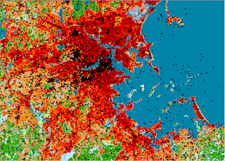
This week we were introduced to MEDS, which stands for Minimum Essential Data Sets. It is a series of minimal essential data sets are critical to the success of a HLS operation.   It consists of the following 8 minimal data sets: Ortho imagery Elevation Hydrography Transportation Boundaries Structures Land cover Geographic Names Due to the data used being critical to safety operations, there are minimal goals for resolution, accuracy, and currency in place for both Urban and Large areas.  For our lab this week, I prepared a MEDS GIS that helps identify key data sets to prepare for a Boston Marathon bombing crisis scenario. Started by organizing a new map based on a Boston Geodatabase. Then created 7 different group layers to include ortho imagery, DEMs, geographic names, transportation, hydrology, boundaries, structures, and land cover data. Given a specific study area helped identify only the Boston Counties affected along with geographic sites. The transpor

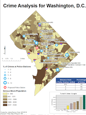
This week we start look at how GIS is used for solving homeland security and law enforcement decisions. This first assignment focuses on how crime is analyzed and managed using GIS by performing a crime analysis for Washington D.C. using data from the DC Metropolitan Police Department . For the first map deliverable, I Geocoded Police Stations from table data in order to create a point shape file for a Police Stations layer. Using a Distance Buffer and Spatial Join for Crime proximity, I was able to determine that higher populated areas do not necessarily mean higher crime rate. However, for some reason, there’s more crimes committed closer to Police stations. A majority of crime tends to occur within 1 mile of Police Stations according to the pattern displayed. Police stations are displayed by percentage of crime activity. The Police Stations with the highest crime percentages are Sixth District (6D), Seventh District (7D), and Third District (3D). 6D observes a lot of theft type

This week's assignment closes our section in natural hazards with Hurricane Sandy. Using data from NOAA, FEMA, and state of New Jersey I was able to first map Hurricane Sandy's path then take a closer look at the damage caused in Ocean County, NJ. The map below was created using table data detailing storm information to create a storm path, which was them symbolized to display how it changed from start to end. I also performed a Storm Damage Assessment using NOAA, FEMA, and state of New Jersey data. The most important step for this assessment was putting together two raster mosaics, one pre-storm and one post-storm, of aerial imagery for the study area. I was able to create a chart of damage done to one side of Fort Ave using the two mosaics and ArcGIS's Effects tool.

This week's lab had us create an evacuation map for the tsunami in Fukushima, Japan. Part of it also served as refresher in best practices for setting up a new Geodatabase using only base data files. Which meant I had to organize different feature classes into feature datasets to improve productivity. There is a lot of data involved for a natural disaster scenario and it drove home the importance of maintaining specific feature datasets within the geodatabase. One of my favorite steps in this lab involved the Fukushima and Sendai area DEMs that helped generate Evacuation Zones 1-3, not pictured in the final map in order to create a final affected coastal zone DEM. I had never created a model as large as the one for this step in model builder, it certainly saved a lot of time. What I've taken away from this scenario is that whichever method of risk assessment is used, the GIS specialist has to be prepared with the data organized and ready to present during an emergency in o

For our first lab of this course we had to identify potential hazard zones for the Mt. Hood area in Oregon.  I was able to create a final stream feature using tools in the  Spatial Analyst Extension in ArcGIS, a 2011 USGS 30M DEM of the region, census block group data, and hydrology data. To do this, I had to convert a number of rasters using the original hydrology data and DEM to determine a flow. Then, using the census block data, I was able to determine which block groups were in hazardous areas based on whether they intersected the hazard stream at .5 a mile buffer. The final result is a population analysis for areas within hazard zones. As one can see, there is a strong concentration of people, cities, and schools Southwest of Mt. Hood.