Julieta's GIS Blog

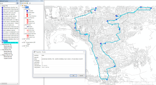
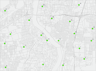
This week in Special Topics in GIS was our first week looking at Networks, we focused on Network Analysis specifically. There were two parts to the lab, the first was a set of introductory exercises to help us refresh on how to create a Network using ArcMap's Network Analyst extension tools as well as review the elements that make up a functioning Network. For the second part of the lab we modified data for provided Network. First I created a new Network Dataset with Turn Restrictions by adding RestrictedTurns and Streets feature classes to the data frame. A point shape file of Facility locations was used for Stops. There were a total of 19 Stops that resulted in a total time of 105.5 Minutes (1.76 hrs). For the final portion of the lab, I created  a second Network Dataset which included a Traffic Model. The Traffic model is enabled in the Network setup wizard and allows your network to use historic traffic data for an analysis. The map below displays the new route and

This week, we revisited our aerial LULC Classification analysis of Pascagoula, Mississippi in order to determine accuracy using ground truthing methods. I created a random sample pattern of points in a new shape file and placed them throughout my previous LULC Classification map layout. Then performed a ground truthing assessment of land features using Google Street Map view online. Accuracy percentages resulted in 57% accurate points and 43% false points. Looking back, I believe I could have done better in my initial assessment of features in the aerial photograph.

In this assignment, we learned how to determine the quality of road networks by determining their completeness by comparing total lengths of two different road data sets. Using Calculate Geometry, in kilometers, I was able to determine that TIGER roads were more complete by comparison. Total TIGER Roads length came out to be 11,383 km, while Street Centerlines were 10,805.8 km. I actually had a more difficult time organizing this analysis than initially expected. The method that seemed to work was to first clip the two roads to the grid shape file. From there run the Intersect tool on both road clips to the grid, separately of course. Then gathered the length info from each road DBF files and added it to a new excel sheet to included GRIDCODE, FID, and Lengths. In this new sheet, I then calculated the percentages using the provided formula of: % difference = (total length centerlines – total length TIGER) / total length centerlines * 100% Then I added this sheet to the TOC

There was a lot of content to digest this week in Photo Interpretation and Remote Sensing. We delved into what Land Use and Land Cover actually represent, and Land Use Land Cover (LULC) classifications, reasons, definitions, and its process. It was very interesting learning about this system's process, the technology required for recording data, and how the recording of data for each type of main feature differed from one another. I hold a personal interest in this field, so it was a fascinating read. The lab required to create a land use/land cover map from a provided aerial photograph by applying recognition elements to LULC classification and be able to identify various different features. I was able to identify 12 unique features. Unfortunately, I ran out of time and did not get to identify all of the features in the aerial photograph.

For this second week into standards in regards to Data Quality, we had to perform a horizontal accuracy assessment using NSSDA protocol methodology in order to determine the accuracy of two different street map data sets based off the same area in Albuquerque, New Mexico. Using two different street sample data sets: City data (ABQ_Streets) and ESRI street map data (StreetMapUSA). I started things off by creating a network data set for each street shape file in ArcMap. Next, in order to be mindful of the study area and attempt to make sure the points met the criteria, I created a fishnet with 2x2 columns/rows which creates 4 quadrants within the study area. Working off the Junction layer for ABQ_Streets, I selected 20 intersection test points as suggested. It was encouraged to use the City data set due to it being more accurate. Then comparing the selected test points, I selected matching test points for the StreetMapUSA data set. The third and final data set needed for this lab w

For this module's lab, we observed three different aerial images for three different purposes: first served to identify tone and textures, second was identifying physical features, and third was interpreting color. Only two maps were required for the first two exercises. The objective for exercise 1 was to be able to identify texture and tone in an aerial photograph. For both elements, it was required to observe at least 5 different tones and textures (i.e. light, very light, dark, coarse, etc.). The objective for exercise 2 was to learn how to identify features according to shape and size, shadows, pattern, and by association. I think I did a good job after zooming in and examining the aerial image closer to try and identify features better. Shadows became very helpful in singling out possible trees or street posts which then helped with associating other features nearby.